

#07 Weekly market update (01/11/2021 - 05/11/2021)

Weekly performance:


Key takeaways:
Economic calendar. CPI data for the US, Eurozone, Canada and the UK will be released next week, which could question the transitory narrative by Central Banks. GDP growth in Japan and the Eurozone will add further evidence of economic recovery. Retail sales in the US, the UK and Canada will show the evolution of consumer trends.
Macroeconomic outlook. Eurozone and US’ Manufacturing PMIs show a worsening situation in the supply chain crisis after reaching an 8 and 19-month lows, respectively. Manheim Used Vehicle Value Index and North America Fertilizer Price Index reach new all-time highs, adding further pressure on inflation. The BoE’s dovish response surprises investors. The Fed will initiate the tapering process in mid-November at $15bn per month. US nonfarm payrolls increased by 531,000 MoM, labour force participation rate remains unchanged at 61.6%. US productivity at its lowest since 1981.
Equities. The Russell 2000 closed the week gaining more than 6%. US equities outperforming the rest of the world developed economies’ indexes since 1997. S&P 500’s Put/Call Ratio at 0.76. 66% of the European companies reporting better-than-expected Q3 earnings (vs. ≈51% historical average).
Fixed Income. Highest inflows in bonds since the first week of September after the dovish interventions from the RBA, Fed and the BoE. The 10Y US Treasury back to the MA 200 ($131.82).
FX. GBP dropped sharply after BoE voted to keep interest rates on hold at 0.1%. Macroeconomic data suggests stronger USD compared to the EUR.
Emerging Markets. The Chinese developer Kaisa, suspended from trading after unprecedented liquidity pressure. China High Yield Index over 20%.
Commodities. YTD best year for commodities since 1973. OPEC rejects Biden’s proposal to increase oil supply, production for the month of December to be increased by 400,000 barrels. Gold seasonality suggests outperformance during the months between November and February.
The economic recovery seems not to be that clear
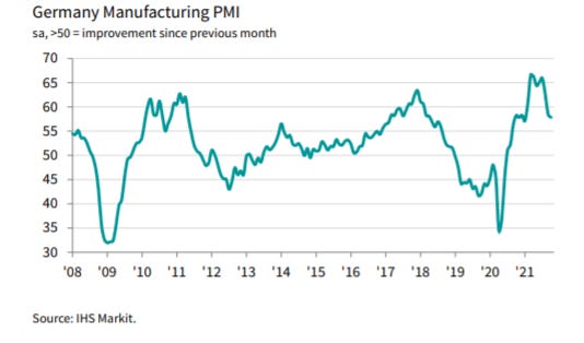
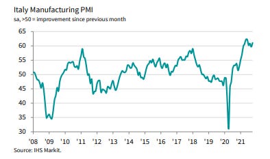
The IHS Markit Manufacturing PMIs for the Eurozone, China and the US have been published this week. Except for Italy and China, all other PMIs (Eurozone, Germany, France, Spain, and the US) have shown a worse-than-expected economic outlook. Figure 1 depicts the Eurozone Manufacturing PMI. As observed, the indicator has dropped to an 8-month low (58.3 Oct. vs. 58.6 Sep.) after EU manufacturers reported a worsening situation in the supply chain crisis. Another takeaway from the survey is the increase in the median delivery date of commodities, as only in two months of the last twenty-five years had been longer. This shortage has allowed suppliers to increase their commodity prices, something which has brought about an increase in the input price index from 86.9 to 89.5, the highest since the date of inception of that indicator. When it comes to Germany, the latest data keeps reflecting material shortages translated into increasing selling prices (Refer to Figure 2). Another country which has struggled to secure raw materials and demand conditions has been France, with its Manufacturing PMI accounting for 53.6, the lowest in the last nine months (See Figure 3). As observed in Figure 4, Spain has witnessed a record deterioration in vendor delivery times in October as inputs remained in short supply. Moreover, output and new orders have risen at the weakest rate since February 2021. The Manufacturing PMI in the US (Refer to Figure 5) has significantly dropped with respect to September (58.4 vs. 60.7 prev.) given the material shortages, which has been the lowest in the last 15 months. Conversely, Italy’s Manufacturing PMI has improved at one of the quickest rates (61.1 vs. 59.7 prev.) despite the persistent supply disruptions (See Figure 6). Other EU countries like Austria or The Netherlands have been on an increasing trend, with the highest Manufacturing PMIs in the last 8 and 2 months, respectively. Finally, as illustrated in Figure 7, China has also faced an improvement in the demand in the last month (50.6 vs. 50.0 prev.). Yet, power shortages and rising costs of production are the main threat to the industrial sector. The severity of the delivery times can be reflected in Figure 8. As observed, Japan is the least affected, but, as the US and the Eurozone, all three regions have a worse outlook than that of the first months of the pandemic. Nonetheless, the UK has not reached the worst scenario yet.


Another striking data released this week has been the US productivity, which is now the lowest since 1981. As observed in Figure 9, US nonfarm business labour productivity has decreased 5% QoQ while unit labour costs have increased 8.3% in that same period. This data supports the already mentioned firms’ rising costs combined with the shortage of labour force. The only solution to this issue is to significantly increase salaries in order to attract employees. An additional detrimental factor is the bottlenecks in the supply chain, which are bringing about increases in PPI and delays in the manufacturing processes. Ultimately, the drop in productivity may be suggesting a wage-price spiral, one of the countless contributors to the persistent inflationary pressures.

Fertilizer prices and Manheim Used Vehicle Value Index increase inflationary pressures
Inflation is undoubtedly on the spotlight, something which seems not to revert soon. Fertilizer prices have been on a parabolic increasing trend since mid-2020 and have reached a new all-time high. Accounting for $1,019.47 per short ton, fertilizer prices are up 43% since June. This rise is harming farmers’ abilities to plant their crop and provide affordable food supply. As a result, retailers are now only buying what they need for the immediate future (See Figure 10).

This week, Gary Schnitkey, an agricultural economist from the University of Illinois has published a paper in which he aims at forecasting the planting and acreage decisions in 2022. He concluded that fertilizer costs in 2022 will be higher for corn and soybeans, with an increasing cost of $100 and $50 per acre, respectively. Regardless of the higher increase in cost for the former, Schnitkey projects corn to be more profitable than soybean in the next year. As observed in Figure 11, from 2013 to 2020, soybean has been outperforming corn.

Similarly, Europe is also adding inflationary pressures by increases in food production costs (Refer to Figure 12). This week, the prices for ammonia in western Europe have reached a new high since 2008 at $910 per metric ton. Affected by the natural gas crunch, Europe has witnessed how a significant number of nitrogen-fertilizer plants have been forced to halt its production. According to Basf SE, gas accounts for 80% of the cost of its nutrient production process. As a result, a prolonged decrease in output could take its toll in food prices.

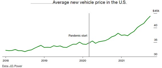
Another important “transitory” component of inflation is transportation, which is being distorted by the Manheim Used Vehicle Value Index. Last week, the indicator reached new all-time high at 223.7, with a monthly increase of 5.5%. Cox automotive has also identified a higher-than-usual sales conversion rate (67% vs. 49% October 2019), which indicates that buyers are being much more aggressive in buying compared to the average October months. (See Figure 13). Figure 14 shows the increasing average price of new vehicles sold in the US. As we can see, the price has almost soared $10,000 an increase of a 28% since the pandemic started. Similarly, Figure 15 depicts the average number of days a new vehicle remains at the dealership until being sold. Before covid, a car sale would take 70 days for an average car dealer. As of today, the same car is being sold in less than 25 days.


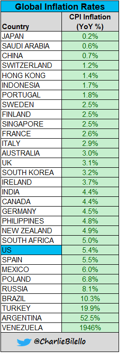
Charlie Bilello, the founder and CEO of Compound Capital Advisors, has published its monthly inflation data across countries. As observed in Figure 16, most countries are suffering from increasing inflationary pressures, while those reporting inflation lower or equal to 2% are the exception, rather than the norm.
US FOMC: Tapering initiates, no rate hike yet
One of the most eagerly awaited moments of the year took place last Wednesday. As expected (and already priced), Jerome Powell announced the tapering, which will initiate by the end of November at a pace of $15 billion per month ending by mid-2022. The Committee stated that chances are monthly asset purchases will be reduced over the months, but they are open to adjust the pace (of purchases) if required by the economic outlook. They reinstated that the Fed will continue to foster smooth market functioning and favourable financial conditions, thereby supporting the flow of credit to households and businesses.
Powell acknowledged the pandemic has delayed the economic recovery and claimed they are constantly the external inflationary and supply chain-related shocks. The Fed has kept reinstating the transitory message. Despite the supply and demand imbalances have brought about an increase in price levels, and consequently, a higher-than-expected CPI, they expect inflation to progressively decrease. The Chair of the Fed stated that he sees inflation decreasing by 2-3% by next semester, an excessively optimistic view in my opinion. When asked about supply chain bottlenecks he expects the problem to persist in 2022 but made clear that the Fed can’t do nothing about it, given it’s out of its two main objectives: Price stability and full employment. Yet, he sees the economy improving, but warned that it may take a while until the situation regularizes to pre-covid levels.
With regards to employment, he acknowledged the labour market participation rates remains low, while emphasizing on both the workers’ deficit and the increasing difficulties faced by companies to retain employees and fill vacancies.
The most important takeaway from the meeting was the dovishness to rate hikes. Despite many investors were expecting a sooner-than-expected increase in the interest rates, the Fed considers we are not in the adequate scenario to make such a decision as the labour market would need to finalize its recovery.
How may the market react to tapering? To put things into perspective, we must go back to 2014, when the Fed last announced a tapering decision. As a response to the 2007-2009 crisis, the Fed started reducing its asset purchases by $15 billion per month from January to October 2014. Conversely, the EU, Japan and many other countries were still stimulating their economies, something which differs to the current outlook as many countries may make the same decision soon. The fact of the Fed is more concerned about inflation than what it used to be some months ago may play in favour of the USD, which may benefit from a rate hike. With regards to bonds, investors similarly expect the Fed to be more hawkish than expected to fight inflation. As a matter of fact, JPMorgan expects 16 of the 31 central banks to have already hiked interest rates by end of the year. As a result, rising yield expectations of a tighter monetary policy and rebounding growth have led to the worst year for US bonds since 2013. Finally, the S&P 500 soared to all-time highs after the Fed’s decision, a reflection of the current scenario.
In my opinion, the question is whether the Fed (same applies to the ECB) is wrong on its “transitory” message on inflation and labour markets. The main reason for the Fed not hiking rates is the labour force, which according to Powell is something difficult to assess given the supply chain disruptions, increasing quit rates and persistent wage pressure. Said in other words, the labour market is already running extremely hot. As observed in the employment data released on Friday (See Figure 17), nonfarm payrolls increased by 531,000 MoM (vs. 450,000 forecast). Similarly, unemployment rate improved from 4.8% to 4.6% with respect to the data from September. Nevertheless, the most important figure is the labour force participation, which remains unchanged at 61.6%.

My view after the FOMC meeting (same rationale applies to the recent dovishness by other major central banks like the RBA, BoE or the ECB) is that the Fed is overconfident in its transitory narrative, as current data shows persistent inflation, especially on the most transitory components namely food and energy. Moreover, the official announcement of the tapering process starting in mid-November at $15 bn/month ($10bn in Treasuries and $5bn in MBS) with a possible swift in that tapering process could mean an increase in the pace of tapering during early 2022 in order to cope with persistent inflation. As a result, this would allow the Fed to raise interest rates several times in 2022. Moreover, 2022 is expected to face a weak credit impulse, especially after the gigantic credit expansion post-Covid. This combination makes a flattener trade a worth considering option.
Despite the massive inflows in fixed income (the highest since the first week of September), which was accentuated after the announcement of the BoE not hiking rates, I still expect a flattening of the USD yield curve. For this reason, my suggested flattener trade idea consists of shorting bonds in the front-end (US 10Y) and simultaneously buying long in the back end (US 30Y). In order to properly execute the suggested trading strategy, we would need both legs of the trade to be hedged, which is accomplished by setting a neutral duration (DV01). The amount of each leg is set by the price ratio provided by CME Group. According to the most recent data, this ratio accounts for 5:2, which means that in order to execute a hedged flattener trade, 250 10Y US Treasuries need to be shorted per every 100 30Y Bonds bought. If preferred there is an alternative trading strategy consisting of short selling 100 futures of the US 30Y-10Y spread through the Chicago Mercantile Exchange (CME), which could be more cost-effective than the former option. Both options are represented in Figure 18.

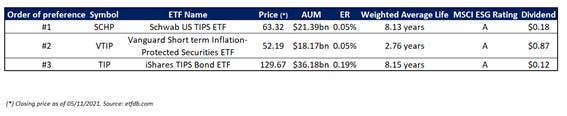
Another recommendation given the persistent inflationary pressures is being heavily invested in TIPS. The most cost-effective way to be exposed to inflation-protected assets would be trough an ETF. In order to decide the most appropriate TIPS investment strategy, I have defined the following criteria: First, I would opt for a long-term ETF rather than a short-term given the high correlation with inflation in the latter. The fact that the former would be uncorrelated with inflation would add diversification to the portfolio and thus, reduce idiosyncratic risk. Finally, I would select the ETF with the lowest expense ratio and highest dividend (if possible). Thus, my recommendation would be to invest in Schwab US TIPS ETF (SCHP). Other ETFs like those owned by Vanguard and iShares would conclude my top three picks (See Figure 19).
In any case, volatility in the bonds market will remain high in the next months as long as the central banking intervention and inflation pressures persist. For this reason, a good hedge would be going long on the Merrill Lynch Option Volatility Estimate (MOVE) Index. Similarly, I personally view the Fed outpacing the ECB in terms of velocity in monetary policy response, something which leads to a stronger USD against the EUR.
Strong momentum for equities, volatility may spike as the option expiry date approaches
As observed in #05 Weekly market update, we are currently immersed into a favourable seasonality for the S&P 500, which runs from October 30th to April 26th. Such a catalyst was also observed by the quant Charlie McElligott, cross-asset macro strategy MD at Nomura. As of November 5th, we can affirm that the favourable seasonality is going according to plan, with the NASDAQ and S&P 500 yielding +2.77% and +1.88%, respectively. Nevertheless, the Russell 2000 Index has been the focus this week with a weekly gain of 6.05%. As observed in Figure 20, the small-cap proxy index has broken the horizontal channel in which it had been stuck since early 2021. This swerve has caught institutional investors’ interest.

In a recent paper by Bank of America, they see the Russell 2000 outperforming big-cap stocks during the next ten years (Currently at 1.5/10), as the small cap companies lagged from 2013 to 2020. Figure 21 depicts the cumulative performance of the S&P 500 vs. the Russell 2000 Index from 2000 to 2009. Moreover, Figure 22 shows how the positive return for the S&P 500 significantly drops when the small caps outperform the S&P 500. They have also observed that the S&P 500 is currently outperforming the rest of developed economies’ indexes since 1997. To put it into perspective, that divergence is currently exceeding 2.3 standard deviations, whomst probability of occurrence is less than 1%. From Figure 23 we can observe how this exuberance has historically reversed after the manias convert into crashes. After the Nifty 50 bubble exploded, the S&P underperformed the rest of the developed economies indexes for more than 20 years. Similarly, the 2000s euphoria brought about ten years of underperformance.


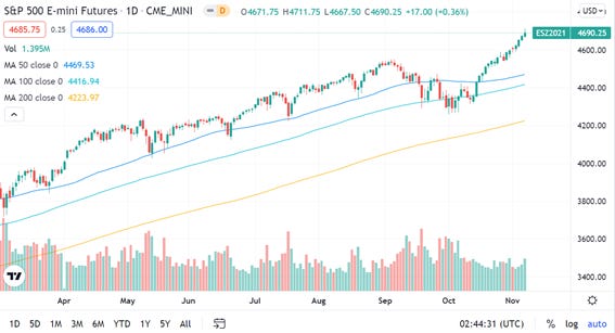
If we have a look at the technical chart of the e-mini S&P 500 (See Figure 24), we can identify the parabolic increase since mid-October, which may find some resistance in the 4,750-4,810 level. The CBOE Total Put/Call Ratio, which is on the verge of crossing 0.75, also shows the increasing bullish sentiment during the last bull run (Refer to Figure 25). According to BofA, its private clients ($3.3 trillion AUM) have reached a new all-time high exposure to equities (65.6%) while cash levels are the lowest since September 2018 (10.6%). When it comes to the blackout period, from Monday onwards all companies will be allowed to repurchase its shares.

We must bear in mind that the option expiry date is November 19th, something which has put obstacles in the S&P 500 performance in the last months. As retail investors buy call options, institutional investors need to buy the underlying asset to hedge the put and, as the expiry date approaches, most calls are out of the money, and thus, institutional investors sell the underlying to undo its hedge. Something to consider for the incoming option expiry day is that the volume of stock options over its underlying shares (in %) has reached an all-time-high (See Figure 26). Following this logic, the market may start preparing for that event from Wednesday onwards. This may be anticipated by the Dark Pool Index (Refer to Figure 27). As observed, institutional investors have been buying during the S&P 500’s strong momentum. Yet, a divergence may be originating given the drop in the DIX on last Friday.


This scenario suggests that a possible future trend may be betting on the outperformance of the world developed economies excluding the US. Some interesting ETFs for pursuing this strategy may be the iShares MSCI EAFE ETF, Vanguard, the FTSE Developed Markets ETF or the iShares Core MSCI EAFE ETF. Weekly performance: CAC40: +2.48%; DAX40: +1.84%; Euro Stoxx 50: +2.49%; FTSE MIB: +2.24%; Nikkei 225: +2.75%.
22nd OPEC and non-OPEC Ministerial meeting: Rejection to Biden’s demand of increased oil supply
Last week, the US President Joe Biden claimed fuel costs being high because of “the refusal of Russia or the OPEC nations to pump more oil”. As a result, oil prices tumbled more than 4% anticipating a possible agreement on increasing supply on the 22nd OPEC meeting. Yet, the OPEC nations emphasized in ensuring a stable and balanced oil market and decided not to increase oil production by sticking to the expected monthly overall production increase of 0.4 mb/d for the month of December 2021 or, said in other words, 400,000 barrels per day. This resolution may force the US, whomst demand is double the expected increase in production in December, to keep making use of its crude stockpiles in order to drive down prices (Refer to Figure 28). The next meeting will take place on 2nd December 2021. Yesterday, the largest oil producer Saudi Aramco announced they are raising the official selling price of all Saudi Arabia Crude Oil by $1.40 to $2.70. Bank of America remains bullish on Brent Crude Oil and expects to reach $120 by June 2022.

Favourable seasonality ahead for gold
As of today, 2021 has been the best performing year for commodities since 1973. Nevertheless, this is not the case for Gold (-6.35% YTD), which not only is underperforming the broad market, but it is also one of the commodities with lower yield. Nevertheless, this trend may reverse given its favourable seasonality between the months of November and February. According to Seasonax, one the most reliable sources for seasonality trends, the noble metal has benefited from a favourable seasonality from mid-November onwards in the last 53 years. After reaching its peak by the end of February, gold then enters a flattening trend (Refer to Figure 29).

Disclaimer: I have done my best to ensure that the information provided on this newsletter is accurate and provide valuable information. Nevertheless, the content is used for illustrative purposes only and does not constitute investment advice.
Before you leave…
I kindly welcome your feedback/suggestions/critics, etc to improve the usefulness of it to you. You can reach me at jramos@u.nus.edu. If you would like to receive the newsletters as they are published please subscribe. I also appreciate if you share it with your friends who are interested in this space. Thank you.